Previous post

We saw previously that the inclusion of a variable that is the consequence of both a plausible cause and the outcome of interest (a collider) may lead to very good prediction models, but which may be more than useless! They can actually be misleading. Our example used a variable, “app usage” that is posterior to the others, pancakes-related variables, and may seem like a too obvious case for the sharp minds of my reader.

A more subtle example: the “M” bias

Let’s move together to another area, for the next case study: public health.

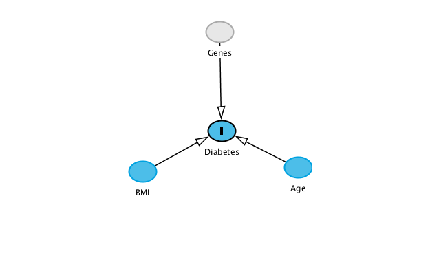
Let’s imagine that the government is ready to put a lot of money to adress the type 2 diabetes issue, and more specifically to prevent the occurrence of type 2 diabetes. But what to act on? Main known (causal) drivers of type 2 diabetes are genetics (non-instrumental), age (non-instrumental) and obesity (already sufficiently adressed, according to the government). Lets find a new interesting, workable feature that leads to type 2 diabetes, that we can act on!

In this fictional scenario, type 2 diabetes is the consequence of genes, age, BMI, and that’s all, so this new driver reseach is destined to find nothing. See figure for the transcription of these hypotheses.

However, the government doesn’t know this, and has access to a lot of data. Thus, it hires a team of Data Scientist in this quest to find a new feature causing type 2 diabetes. In the government data set, from extensive interview of random individuals, there is data on whether one’s mother has diabetes, or not, as well as, why not: one’s number of opera visit during childhood. Both totally non-causal with respect to one’s diabetes status. However, both are statistically related to one’s diabetes status, as described by the next DAG: mother’s genes influence mother’s diabetes status, as well as one’s diabetes status (because it influences one’s gene), but we don’t have genetic data on the government database. Moreover, family income is causing both mother’s diabetes (because it impacts mother’s BMI) and number of opera visit during childhood, but we don’t have access to childhood income either.

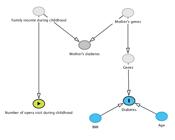
Similarly as in the previous post, data is generated following this last DAG, and we are going to perform predictions, to find if other features predict diabetes.

Again, we build several models to predict the diabetes risk, using all available data: age, bmi, mother’s diabetes status and number of opera visits during childhood. On the contrary to the previous analysis, all variables precede the outcome. The results in terms of AUC are below:

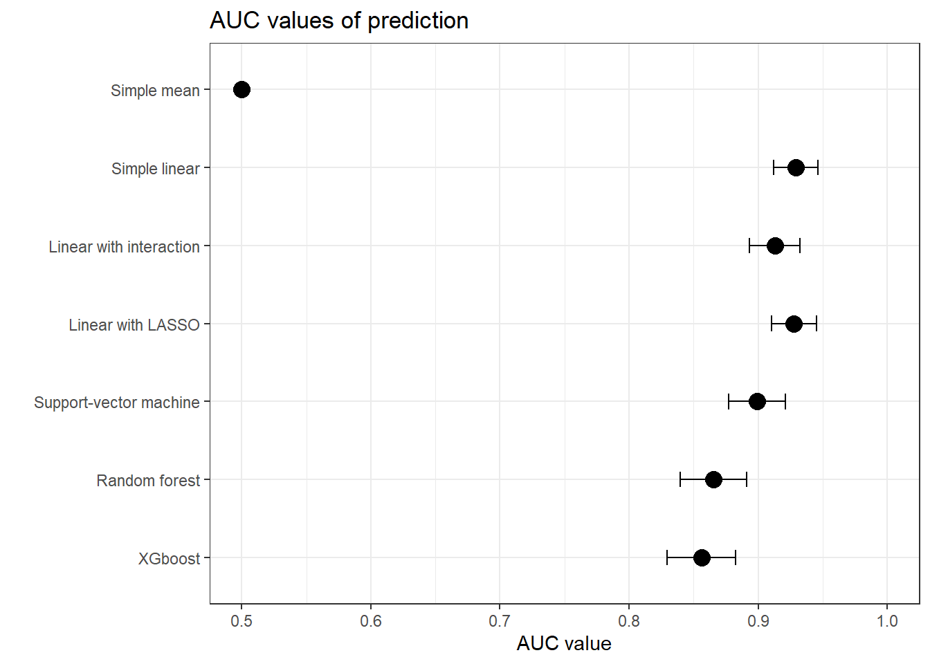
Figure 1: Performances of diabetes prediction

Great, we have again excellent predicting models, such as the simple linear model. With it, we are able to predict diabetes with a discriminatory power (AUC) of 0.93, for the linear model!

Let’s look at the relationship between the only operational variable (number of opera visits), and the predicted risk of diabetes, in the best model that we obtain, for a mean individual.

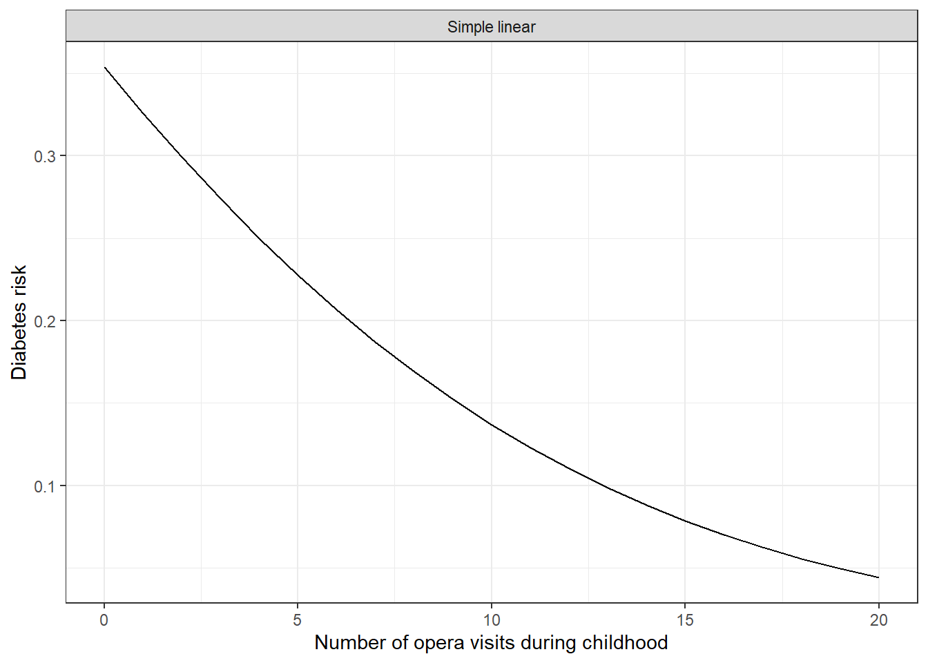
Figure 2: Predicted risks of diabetes

Amazing; our awesome predicting model tells us that the diabetes risk decreases with the number of opera visits during childhood. From 35% diabetes risk for individuals who never had the chance to visit the opera during childhood, to less than 5% risk for lucky ones with more that 20 opera visits!

The Data Science team reports to the government, that decides to found a national plan for Opera promotion for the youth, hoping to tackle the diabetes issue. Obviously, it isn’t going to be a success.

Whereas a Data Scientist who is aware of causal inference, who draws DAGs, reads Hernàn and Pearl, will identify the “M-bias” from the previous DAG. By including the “mother diabetes status” in a model, according to the D-separation rules, a path is open between the number of opera visits (or any marker of family income during childhood) and diabetes, as long as we can’t include the “genes” variable (that are often not available).

The answer here is thus to remove the “mother diabetes status” from the analysis, leading to less accurate prediction models (because we loose the indirect informations regarding genes status of our individuals) but more accurate causal model, exactly what we want in our settings. In such settings, the effects of age and BMI remains correctly estimated, and the effect of number of opera visits on diabetes falls to null (OR=1.05, 95%CI 0.97-1.13).

Perspectives on causal inference & machine learning

Of course, causal inference doesn’t prevent the use of machine learning. It is mainly an injunction to reflect on the goal of the analysis, on the study design and the meaning of features.

Actually, there are several causal methods using state-of-the-art machine learning algorithms to improve the accuracy of causal inference results. The Targeted Maximum Likelihood Estimation method (Laan and Rubin (2006)) and the Double/Debiased Machine Learning framework (Chernozhukov et al. (2018)) are two very good examples, aiming to estimate point treatment effects, using semi-parametric approach and machine learning algorithms of your choice to predict both of the nuisance parameters (the outcome, and the probability of treatment). Both algorithms are fascinating and are starting to see a widespread use, but their description will be in a future blogpost; see Díaz (2019) for a good first introduction.

References