In brief

A very good prediction model may be useless, or even worse! When trying to evaluate the effect of an action, such as the counterfactual intervention, a prediction model with very good performances can be misleading.

This issue arises from the “fundamental problem of Data Science”: to explain or to predict? This distinction has been described by Pearl and Mackenzie (2018) as well as by Hernán et al. (2019): description, prediction, or causal inference. Data Science is a powerful tool to test causal hypotheses using models & data, or to predict the outcome of new observations with smallest error possible. But both goals may be contradictory: explanatory analysis aims at minimizing the bias term, in the bias-variance decomposition of the error (Shmueli (2010)):

\[ Mean\ Squared\ Error = E[(y_{observed} - f(x_{observed}))^2] = \] \[ Bias(f)^2 + Var(f) + \sigma^2 \]

Minimizing the bias term seeks to obtain the most accurate representation of the underlying theory, often by using interpretable, usually parametric, model . On the other hand, prediction modeling seeks to minimize the bias + variance, to achieve a tradeoff between underfitting and generalization.

As a result, trying to “explain” from a prediction model may lead to wrong conclusions, as we’ll show with some examples.

A first simple example

Once upon a time, there was a startup that sold pancakes.

Strawberry Pancakes Yum, by Flo Karp, 2018

Blossoming, the young pancake start-up (“Pancup”) decided to use Data Science to help target individuals that were the more likely to become loyal customers. They designed a the pancake app (“Pancapp”). They launched a global campaign to gather data, reaching out social media and usual customers, for them to use the app. The goal of the Pancup is to identify who is more likely to be a loyal customer of their company, for example to target future marketing campaigns.

We are using the following DAG to represent that process.

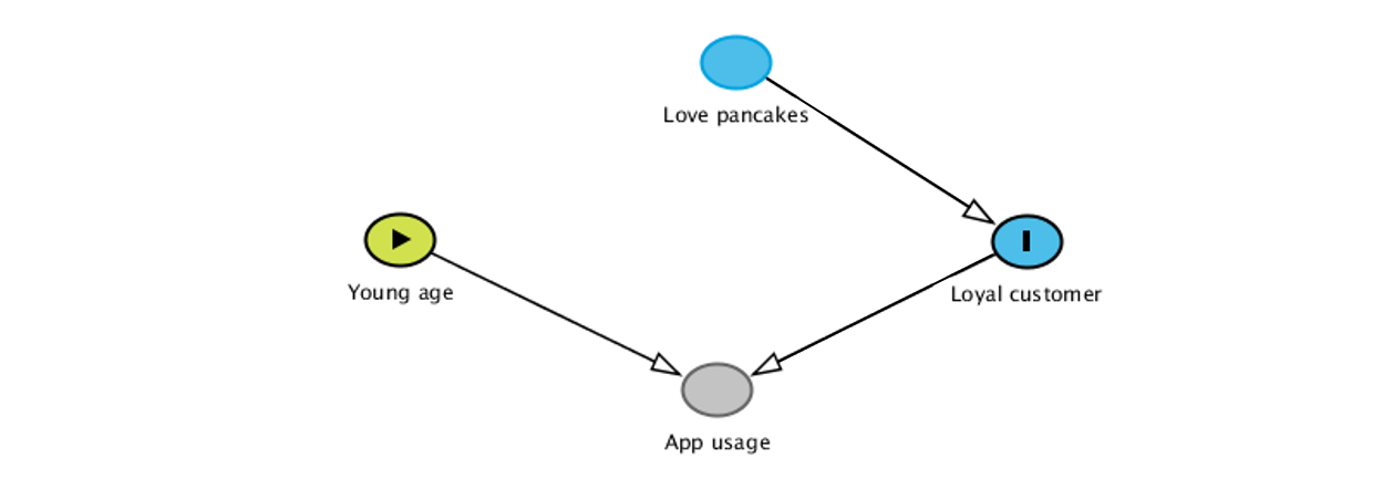
“App usage” represents how much the individuals are using the pancake app. In that simulation, there is no causal link between age and liking pancakes (everybody loves them!), but more importantly, age doesn’t impact the probability of being a loyal customer. Age only impacts app usage, as younger individuals are more easily reached on social networks.

We are simulating the corresponding data with simple gaussian distributions (for age, errors, etc.) and sampling with the following probabilities:

\[ P(Loving\ pancakes)=0.75 \] \[ P(Being\ loyal\ customer | Love\ pancakes)=0.80 \] \[ P(Being\ loyal\ customer | \overline{Love\ pancakes})=0.15 \] Finally, the app usage is an (arbitrary) score determined by age and being a loyal customer or not, plus gaussian noise:

\[ App\ usage= 0.5*age\ +\ \mathbb{1}_{Being loyal customer} + \epsilon \]

\[ \epsilon \sim Norm(0, \sigma^2) \]

The next step is to build a fancy prediction model to predict who are the loyal customers. To do so, we are going to use prediction algorithms on the simulated data, forgetting about the DAG and the process that generated the data.

We use several algorithms, from simple logistic regression, to random forest and XGBoost, to predict the chance of being a loyal customer. We use all available data: pancake enthusiasm, age, and app usage. The figure below ( 1) displays the results, using the “AUC” values, that is a simple discrimination metric (corresponding to the probability that the model will score a randomly chosen positive class higher than a randomly chosen negative class).

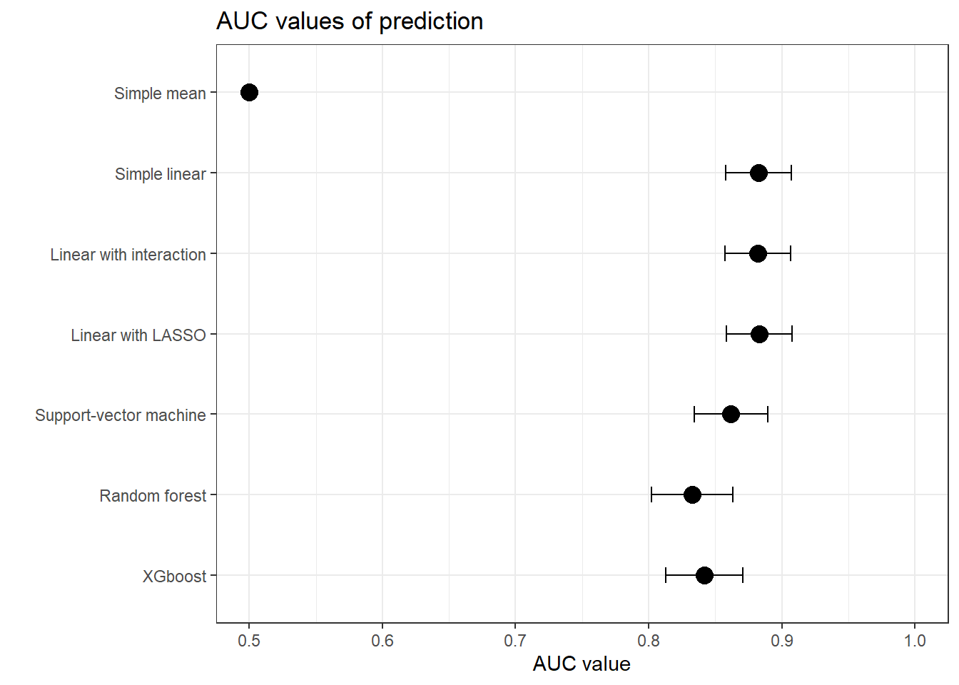
Figure 1: Performances to predict being a customer

In our settings, we see that:

• The “simple mean” model, that uses the mean risk in the train data to predict the risk in the test data, scores similarly to a random classifier, as expected.

• The linear models (logistic regressions) score higher than the more advanced ones - no surprise here, the data-generation process is simple and linear. We note that, still, SVM, random forest and XGBoost hold their own.

Okay, let’s use our models to answer the question: who should we target in future marketing campaigns, who could be more likely to be a customer of the company?

On figure 2 we see the predicted risk of being a customer, depending on the two workable variables, age and liking of pancake, for each of the (interesting) model.

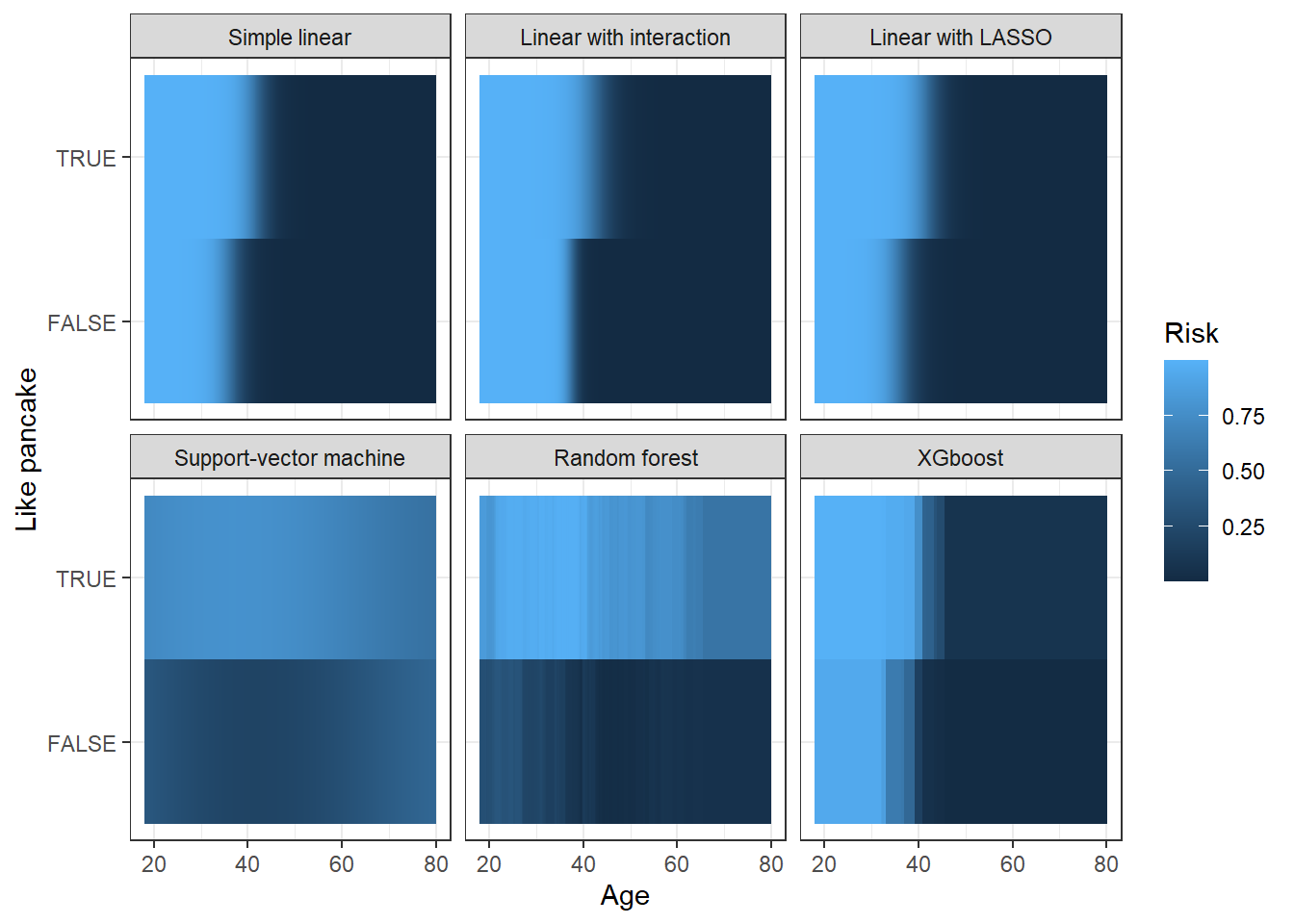
Figure 2: Predicted risks of being a customer

All of the model are in agreement: individuals who like pancakes have a higher risk of being customers, and individuals with a younger age are also found to have with higer risk of being customers, independently of if they like pancakes or not. For example, using the easily interpretable linear model, being 10 years younger increases the odd of being a customer by a factor of 1.57 (1.44-1.72). This result is in contradiction with the reality, with the way we generated our data. Indeed, age doesn’t impact the risk of being a customer, only pancake liking does.

As a consequence, when the company is designing its next marketing campaign, it risks targeting the young people. It means it will loose resources, focusing on a group that doesn’t have higher probability of being their customer, and will do so, no matter how accurate the prediction model is.

However, a Data Scientist aware of causal inference knows that this isn’t a prediction task, but a causal one, that we are trying to identify levers of action. To do so, it is crucial to draw a DAG that summarizes how the data is collected (such as the previous DAG). Using D-separation rules (see Hernán and Robins (2022) or Pearl and Mackenzie (2018)), we see that including “web app usage” in any model will create a spurious link between age and being a loyal customer, as it is a collider of those two variables.

Re-performing the previous analyses, without including the “app usage” variable in the train data, leads to lower performances of the predictive model, as expected.

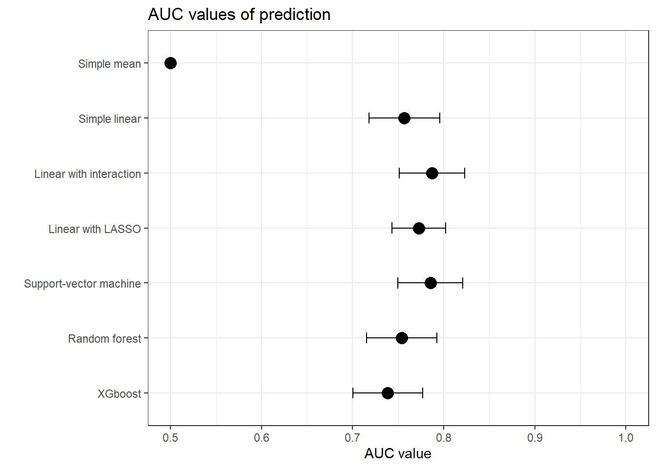
Figure 3: Performances to predict being a customer, from DAG

However, with those models, individuals who like pancakes have a higher risk of being customers, and only them. Age doesn’t impact risk of being customers anymore (or non-significantly so, for the Random Forest & XGBoost).

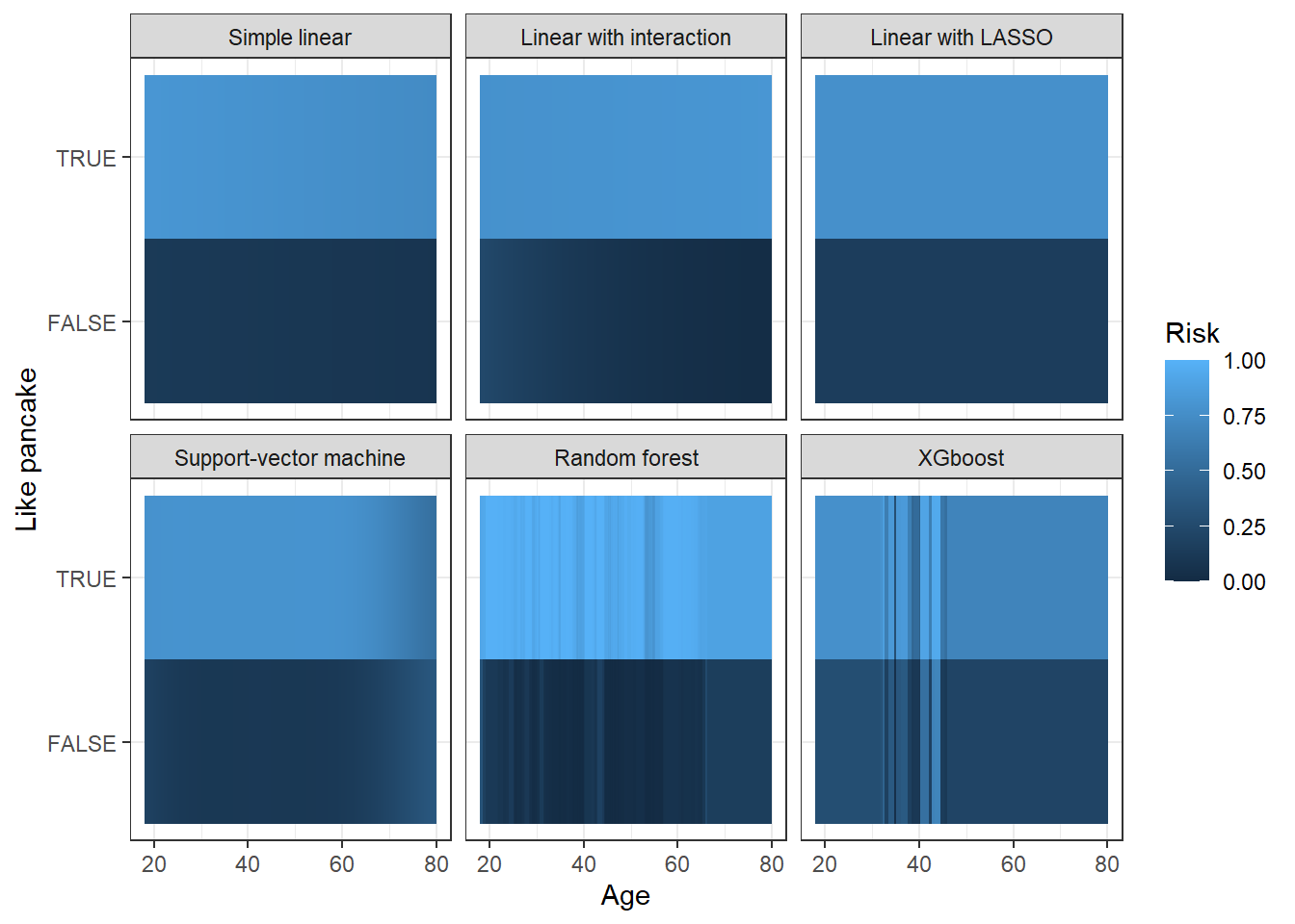
Figure 4: Predicted risks of being a customer, from DAG

As a consequence, the last models provide valuable insight for customer targeting, despite lower performances, thanks to causal inference theory.

It could seem a too obvious example, because the problematic models include a variable that is posterior to the outcome variable (app usage comes after the likeliness of being a customer). However, it does exist more subtle examples of the importance of causal inference, versus prediction methods, when evaluating the effect of an action. See the next post!

References